Central Limit Theorem with JMP

What is Central Limit Theorem?

The Central Limit Theorem is one of the fundamental theorems of probability theory. It states a condition under which the mean of a large number of independent and identically-distributed random variables, each of which has a finite mean and variance, would be approximately normally distributed. Let us assume Y1, Y2 . . . Yn is a sequence of n i.i.d. random variables, each of which has finite mean μ and variance σ2, where σ2 > 0. When n increases, the sample average of the n random variables is approximately normally distributed, with the mean equal to μ and variance equal to σ2/n, regardless of the common distribution Yi follows where i = 1, 2 . . . n.

Independent and Identically Distributed

A sequence of random variables is independent and identically distributed (i.i.d.) if each random variable is independent of others and has the same probability distribution as others. It is one of the basic assumptions in Central Limit Theorem. Consider the law of large numbers (LLN)—It is a theorem that describes the result of performing the same experiment a large number of times. According to the LLN, the average of the results obtained from a large number of trials should be close to the expected value, and will tend to become closer as more trials are performed. The following example will explain this further.

Central Limit Theorem Example

Let us assume we have 10 fair die at hand. Each time we roll all 10 die together we record the average of the 10 die. We repeat rolling the die 50 times until we will have 50 data points. Upon doing so, we will discover that the probability distribution of the sample average approximates the normal distribution even though a single roll of a fair die follows a discrete uniform distribution. Knowing that each die has six possible values (1, 2, 3, 4, 5, 6), when we record the average of the 10 dice over time, we would expect the number to start approximating 3.5 (the average of all possible values). The more rolls we perform, the closer the distribution would be to a normal distribution centered on a mean of 3.5.

Central Limit Theorem Application

• Use the sample mean to estimate the population mean if the assumptions of Central Limit Theorem are met
• Use standard error of the mean to measure the standard deviation of the sample mean estimate of a population mean
• Use a larger sample size, if economically feasible, to decrease the variance of the sampling distribution. The larger the sample size, the more precise the estimation of the population parameter. Use a confidence interval to describe the region which the population parameter would fall in. The sample distribution approximates the normal distribution in which 95% of the data stays within two standard deviations from the center. Population mean would fall in the interval of two standard errors of the mean away from the sample mean, 95% of the time

Confidence Interval

The confidence interval is an interval where the true population parameter would fall within a certain confidence level. A 95% confidence interval, the most commonly used confidence level, indicates that the population parameter would fall in that region 95% of the time or we are 95% confident that the population parameter would fall in that region. The confidence interval is used to describe the reliability of a statistical estimate of a population parameter.
The width of a confidence interval depends on the:

• Confidence level—The higher the confidence level, the wider the confidence interval
• Sample size—The smaller the sample size, the wider the confidence interval
• Variability in the data—The more variability, the wider the confidence interval

JMP: Calculate the Confidence Interval of the Mean

Data File: “CentralLimitTheorem.jmp"

Steps to calculate the confidence interval of the Mean in JMP:

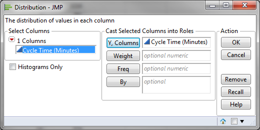
1. Click Analyze -> Distribution
2. Select “Cycle Time (Minutes)” as the “Y, Columns”
   
3. Click “OK”
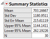
4. “Upper 95% Mean” and “Lower 95% Mean” at the bottom of the newly generated window are the upper and lower boundaries of 95% confidence interval
   

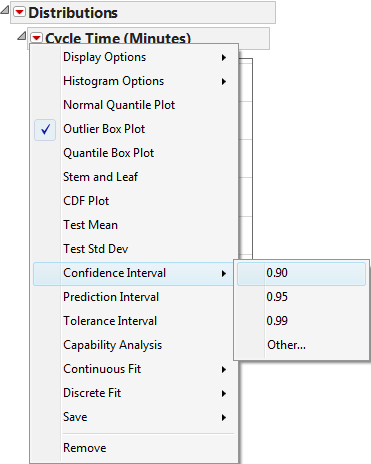
In JMP, the confidence level is 95% by default. To see the confidence interval of “Cycle Time (Minutes)” at other confidence levels, we need to:

1. Click on the red triangle button next to “Cycle Time (Minutes)”
2. Select Confidence Interval -> the confidence level of interest (e.g. 90%, 95%, 99% etc.)
3. The confidence interval at the selected confidence level appears at the bottom of the distribution analysis page