Multiple Linear Regression with SigmaXL

What is a Multiple Linear Regression with SigmaXL?

the Multiple Linear Regression with SigmaXL is a statistical technique to model the relationship between one dependent variable and two or more independent variables by fitting the data set into a linear equation.
The difference between simple linear regression and multiple linear regression:

• Simple linear regression only has one predictor.
• Multiple linear regression has two or more predictors.

Run a Multiple Linear Regression with SigmaXL

Case study: We want to see whether the scores in exam one, two, and three have any statistically significant relationship with the score in final exam. If so, how are they related to final exam score? Can we use the scores in exam one, two, and three to predict the score in final exam?
Data File: “Multiple Linear Regression” tab in “Sample Data.xlsx.”

Step 1: Determine the dependent and independent variables, all should be continuous. Y (dependent variable) is the score of final exam. X₁, X₂, and X₃ (independent variables) are the scores of exam one, two, and three respectively. All x variables are continuous.

Step 2: Start building the multiple linear regression model

1. Select the range of independent and dependent variables in Excel.
2. Click SigmaXL -> Statistical Tools -> Regression -> Multiple Regression
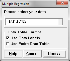
3. A new window named “Multiple Regression” pops up and the selected range appears automatically in the box below “Please select your data”
   
4. Click “Next >>”
5. A new window also named “Multiple Regression” pops up
6. Select “FINAL” as “Numeric Response (Y)” and “EXAM1”, “EXAM2” and “EXAM3” as “Continuous Predictor (X)”
   
7. Click “OK>>”
8. The regression analysis results appear in the newly generated spreadsheet “Multiple Regression” and the residual analysis results appear in another new spreadsheet “Mult Reg Residuals (1)”.

Step 3: Check whether the whole model is statistically significant. If not, we need to re-examine the predictors or look for new predictors before continuing.

• H₀: The model is not statistically significant (i.e., all the parameters of predictors are not significantly different from zeros).
• H₁: The model is statistically significant (i.e., at least one predictor parameter is significantly different from zero).

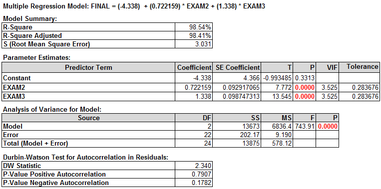
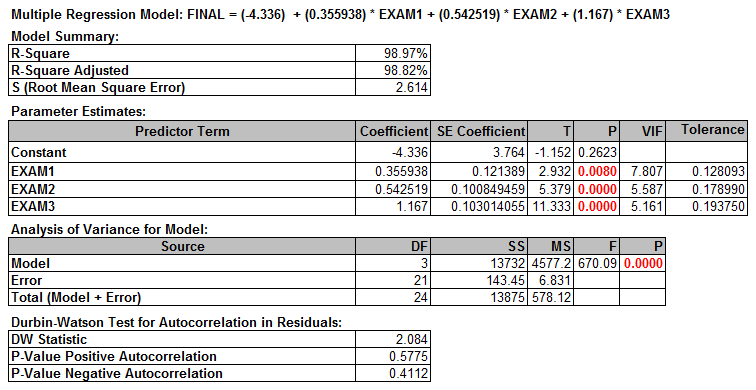
In this example, p-value is much smaller than alpha level (0.05), hence we reject the null hypothesis; the model is statistically significant.

Step 4: Check whether multicollinearity exists in the model.

The VIF information is automatically generated in table of parameter estimates.
We use the VIF (Variance Inflation Factor) to determine if multicollinearity exists.

Multicollinearity

Multicollinearity is the situation when two or more independent variables in a multiple regression model are correlated with each other. Although multicollinearity does not necessarily reduce the predictability for the model as a whole, it may mislead the calculation for individual independent variables. To detect multicollinearity, we use VIF (Variance Inflation Factor) to quantify its severity in the model.

Variance Inflation Factor (1)

VIF quantifies the degree of multicollinearity for each individual independent variable in the model.

VIF calculation:

Assume we are building a multiple linear regression model using p predictors.

Two steps are needed to calculate VIF for X₁.

Step 1: Build a multiple linear regression model for X₁ by using X₂, X₃ . . . X_p as predictors.

Step 2: Use the R² generated by the linear model in step 1 to calculate the VIF for X₁.

Apply the same methods to obtain the VIFs for other Xs. The VIF value ranges from one to positive infinity.

Variance Inflation Factor (2)

Rules of thumb to analyze variance inflation factor (VIF):

• If VIF = 1, there is no multicollinearity.
• If 1 < VIF < 5, there is small multicollinearity.
• If VIF ≥ 5, there is medium multicollinearity.
• If VIF ≥ 10, there is large multicollinearity.

How to Deal with Multicollinearity

1. Increase the sample size.
2. Collect samples with a broader range for some predictors.
3. Remove the variable with high multicollinearity and high p-value.
4. Remove variables that are included more than once.
5. Combine correlated variables to create a new one.

In this section, we will focus on removing variables with high VIF and high p-value.

Step 3: Deal with multicollinearity:

1. Identify a list of independent variables with VIF higher than 5. If no variable has VIF higher than 5, go to Step 6 directly.
2. Among variables identified in Step 5.1, remove the one with the highest p-value.
3. Run the model again, check the VIFs and repeat Step 5.1.

Note: we only remove one independent variable at a time.

In this example, all three predictors have VIF higher than 5. Among them, EXAM1 has the highest p-value. We will remove EXAM1 from the equation and run the model again.

Run the new multiple linear regression with only two predictors (i.e., EXAM2 and EXAM3).
Check the VIFs of EXAM2 AND EXAM3. They are both smaller than 5; hence, there is little multicollinearity existing in the model.

Step 4: Identify the statistically insignificant predictors. Remove one insignificant predictor at a time and run the model again. Repeat this step until all the predictors in the model are statistically significant.

Insignificant predictors are the ones with p-value higher than alpha level (0.05). When p > alpha level, we fail to reject the null hypothesis; the predictor is not significant.

• H₀: The predictor is not statistically significant.
• H₁: The predictor is statistically significant.

As long as the p-value is greater than 0.05, remove the insignificant variables one at a time in the order of the highest p-value. Once one insignificant variable is eliminated from the model, we need to run the model again to obtain new p-values for other predictors left in the new model. In this example, both predictors’ p-values are smaller than alpha level (0.05). As a result, we do not need to eliminate any variables from the model.

Step 5: Interpret the regression equation

The multiple linear regression equation appears automatically at the top of the session window. “Parameter Estimates” section provides the estimates of parameters in the linear regression equation. Now that we have removed multicollinearity and all of the insignificant predictors, we have the parameters for the regression equation.

Interpreting the Results

Rsquare Adj = 98.4%

• 98% of the variation in FINAL can be explained by the predictor variables EXAM2 & EXAM3.

P-value of the F-test = 0.000

• We have a statistically significant model.

Variables p-value:

• Both are significant (less than 0.05).

VIF

• EXAM2 and EXAM3 are both below 5; we’re in good shape!

Equation: −4.34 + 0.722*EXAM2 + 1.34*EXAM3

• −4.34 is the Y intercept, all equations will start with −4.34.
• 722 is the EXAM2 coefficient; multiply it by EXAM2 score.
• 34 is the EXAM3 coefficient; multiply it by EXAM3 score.

Let us say you are the professor again, and this time you want to use your prediction equation to estimate what one of your students might get on their final exam.

Assume the following:

• Exam 2 results were: 84
• Exam 3 results were: 102

Use your equation: −4.34 + 0.722*EXAM2 + 1.34*EXAM3

Predict your student’s final exam score:

−4.34 + (0.722*84) + (1.34*102) =−4.34 + 60.648 + 136.68 = 192.988

Model summary: Nice work again! Now you can use your “magic” as the smart and efficient professor and allocate your time to other students because this one projects to perform much better than the average score of 162. Now that we know that exams two and three are statistically significant predictors, we can plug them into the regression equation to predict the results of the final exam for any student.