Fractional Factorial Designs with JMP

What Are Fractional Factorial Experiments?

In simple terms, a fractional factorial experiment is a subset of a full factorial experiment.

• Fractional factorials use fewer treatment combinations and runs
• Fractional factorials are less able to determine effects because of fewer degrees of freedom available to evaluate higher order interactions
• Fractional factorials can be used to screen a larger number of factors
• Fractional factorials can also be used for optimization

Why Fractional Factorial Experiments?

To run a full factorial experiment for k factors, we need 2^k unique treatments. In other words, we need resources that can afford at least 2^k runs.

With k increasing, the number of runs required in full factorial experiments rises dramatically even without any replications, and the percentage of degrees of freedom spent on the main effects decreases. However, the higher order interactions (3 or 4 factor interactions) can typically be ignored, which allows us to run fewer trials to understand the main effects and two-way interactions.

The main effects and two-way interaction are the key effects we need to evaluate. The higher order the interaction is, the more we can ignore it.

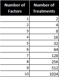
Notice the number of treatments increases dramatically as factors are added.

How Does a Fractional Factorial Work?

We are trying to find the cause-and-effect relationship between a response (Y) and three factors (factor A, B, and C) and their interactions (AB, BC, AC, and ABC). As follows is the 2³ full factorial design (2 level 3 factor). There are eight treatment combinations (2 * 2 * 2).

To perform a 2³ full factorial experiment, we need to run at least eight unique treatments (2 * 2 * 2).
What if we only have enough resources to run four treatments?
As a result, we need to carefully select a subset from the eight treatments so that all of our main effects can be evaluated and the design can be kept balanced and orthogonal.

Example of an invalid design

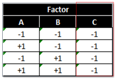
This design is invalid because only the low setting of factor C is tested. We cannot evaluate the main effect of factor C using this design. Remember orthogonality?

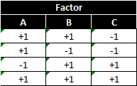
This design is also invalid because it is neither balanced nor orthogonal. Checking orthogonality: the sum of AC interaction signs should equal zero (0).

• Run 1 (−)
• Run 2 (−)
• Run 3 (−)
• Run 4 (+)
• Sum (−1)

This design has a low and high setting for each factor, but is not orthogonal. To select the four treatments run in the 2³⁻¹ fractional factorial experiment, we start from the 2² full factorial design of experiment. If we replace the two-way interaction (AB) column with the factor C column, the design will be valid.

Imagine a two-factor full factorial with factors A and B. We also learn about the interaction of A and B. In a fractional factorial, we sacrifice learning about the two-way interaction between A and B, and substitute factor C.

2³⁻¹ Fractional Factorial Design Pattern

This pattern implies three factors and four treatments.

Note: We also call this kind of design a half-factorial design since we only have half of the treatments that we would have in a full factorial design. In 2³⁻¹ fractional factorial design of experiment, the effect of three-way interaction (ABC) is not measurable since it only has “+1”.
In four runs, we are able to run high and low settings for each of the three factors. The three-way interaction ABC is only at the high setting. In the 2³⁻¹ fractional factorial design, we notice that the column of each main effect has identical “+1” and “−1” values with one two-way interaction column.

• A and BC
• B and AC
• C and AB

In this situation, we say that A is aliased with BC or A is the alias of BC. By multiplying any column with itself, we obtain the identity (I).

A*A=I

The product of any column and the identity is the column itself.

A*I=A

Column ABC is called the generator. By multiplying any column with the generator, we obtain its alias.

A*ABC=(A*A)*BC=I*BC=BC

Use JMP to Run a Fractional Factorial Experiment

Step 1: Initiate the experiment design

1. Click DOE -> Classical->Screening Design
2. A window named “DOE – Screening Design” pops up.
3. One response: Y
4. Add Three factors: A, B and C by clicking the “Categorical” button-> 2-Level, rename the factors, A, B and C
5. Two-level design: each factor has two settings, -1 and +1
6. Click “Continue”
7. Select “Choose from a list of Fractional Factorial Designs”, click “Continue”.
8. Select “Fractional Factorial” and click “Continue”
   

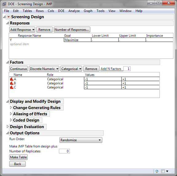
Step 2: Select the number of replications, make design

1. In this case, we want each treatment to be run twice so that there are enough degrees of freedom to analyze the effects.
2. Enter “1” in the box for “Number of Replicates”
3. Click “Make Table” button
   

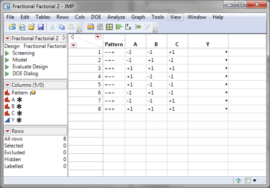
Step 3: Implement the experiment and record the results in the table. For this lesson, use the data file “Fractional Factorial.jmp” with the ‘Y’ data already entered. If you do not use this file then you may not get the same results displayed during this lesson.

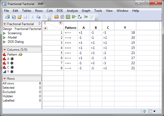
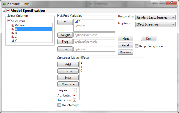
Step 4: Fit the model using the experiment results

1. Click Analyze-> Fit Model
2. The Y and the Xs have been pre-populated into their boxes
3. Click “Run Model”
   

Step 5: Analyze the model results

1. Click on the red triangle next to “Response Y”
2. Select “Regression Reports -> “Summary or Fit”
3. Select “Regression Reports -> “Analysis of Variance”
4. Check whether the model is statistically significant.
5. Check which factors are insignificant.
6. If any independent variables are not significant, remove them one at a time and rerun the model until all the independent variables in the model are significant.
   

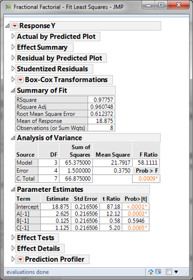
Step 6: The p-value of factor B is greater than the alpha level (0.05), so it is not statistically significant. Next we need to remove factor B and re-run the model.

1. Click the red triangle next to “Response Y”
2. Select “Model Dialog”
3. Remove Factor B from the model
4. Click “Run”
   

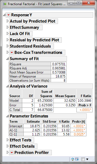
The p-values of all the independent variables are smaller than 0.05. There is no need to remove any independent variables from the model.

Perform residual analysis to ensure that the model's residuals satisfy the following criteria.

• Mean is equal to zero.
• Normally distributed
• Independent
• Equal variance across the fitted response values

Step 7: Save residuals generated by the model

1. Click on the red triangle button next to “Response Y”
2. Click Save Columns -> Residuals
3. A new column of residuals will appear in the data table
   

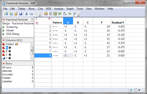
Step 8: Check whether residuals are normally distributed with a mean equal to zero.

1. Click Analyze -> Distribution
2. Select “Residual Y” in the “Y, Columns”
   
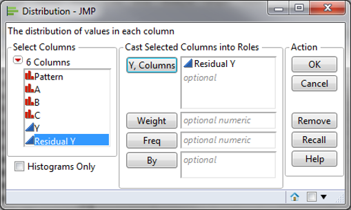
3. Click “OK”
4. Click on the red triangle button next to “Residual Y”
5. Click Continuous Fit -> Normal
6. Click on the red triangle button next to “Fitted Normal”
7. Click “Goodness of Fit”
   

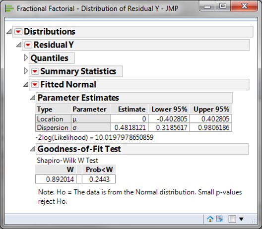
If the p-value of the normality test is greater than the alpha level (0.05), the residuals are normally distributed.

Step 8: Check if the residuals are independent.

1. Click Analyze -> Quality & Process -> Control Chart -> IR
2. Select “Residual Y” as “Process”
   
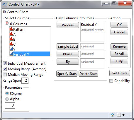
3. Click “OK”
4. I-MR chart of residuals are generated.
5. Click on the red triangle button next to “Individual Measurement of Residual Tastiness”
6. Click Tests -> All Tests
7. If no data points on the control charts fail any tests, the residuals are in control and independent of each other.
   
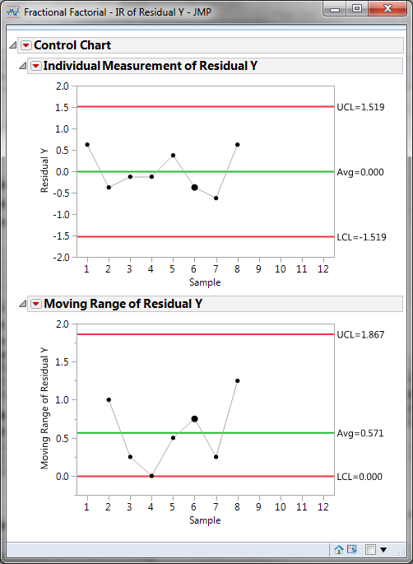
   Note: The prerequisite of plotting an IR chart for residuals is that the residuals are in time order.

Step 9: Check whether the residuals have equal variance across the predicted response values.

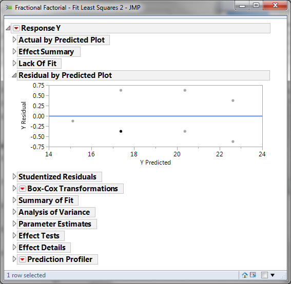
• Within the analysis results page of fitting the DOE model is the “Residual by Predicted Plot”
• We look for patterns in which the residuals tend to have even variation across the entire range of the fitted response values