The normal distribution is also known as a Gaussian distribution. It is the most frequently referenced distribution and approximates many natural data tendencies. The normal distribution is a probability distribution of a continuous random variable whose values spread symmetrically around the mean.

A normal distribution can be completely described by using its mean (μ) and variance (σ2) because mean and variance determine the shape of the distribution. When a variable x is normally distributed, we denote:

x ~ N(μ, σ²)

The probability density function of the normal distribution is:

Characteristics of the Normal Distribution

Shape of Normal Distribution

• A normal distribution's probability density function curve is “bell” shaped.
• All normal distributions are symmetric and have bell-shaped density curves with a single peak.
• Location of Normal Distribution.
  • The mean, median, and mode will have the same approximate values if a data sample or population is normally distributed.
  • The probability density curve of the normal distribution is symmetric around a center value, which is the mean, median, and mode.
• Spread of Normal Distribution.
  • The spread or variation of normally distributed data can be described using variance or standard deviation.
  • The smaller the variance or standard deviation, the less variability in the data set.
• Empiricle Rule: 68-95-99.7 Rule.

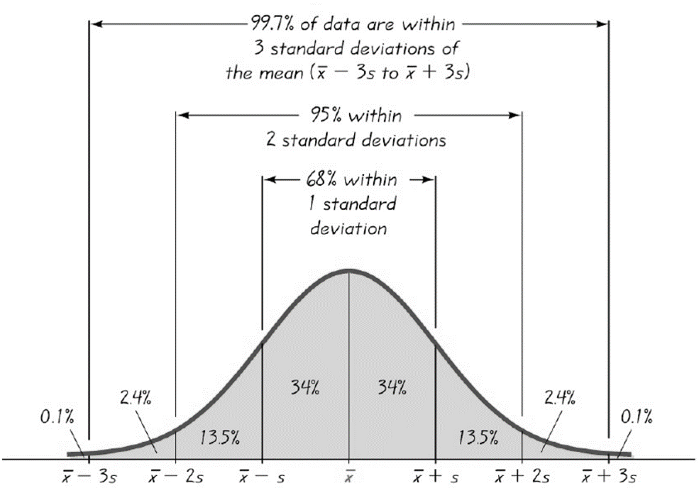
The 68-95-99.7 rule, or the Empirical rule in statistics, states that for a normal distribution.

• About 68% of the data fall within one standard deviation of the mean, that is, between μ-σ and μ+σ.
• About 95% of the data fall within two standard deviations of the mean, that is, between μ-2σ and μ+2σ.
• About 99.7% of the data fall within three standard deviations of the mean, that is, between μ-3σ and μ+3σ.
• The image below depicts this rule:

Normality

Not all distributions with a “bell” shape are normal, so we need to check whether the data are normally distributed. To do so, we should run a normality test. There are different normality tests available.

• Anderson-Darling test
• Shapiro-Wilk test
• Jarque-Bera test
• Normality Testing

Normality tests determine whether the population of interest is normally distributed. As discussed above, several normality tests are available, like the Anderson-Darling test, the Sharpiro-Wilk test, the Jarque-Bera test, and so on. For any of these tests, the null and alternative hypotheses are generally the same:

• Null Hypothesis (H₀): The data are normally distributed.
• Alternative Hypothesis (H_a): The data are not normally distributed.

Use Minitab to Run a Normality Test

Steps to run a normality test in Minitab. (Open normality.mtw using Minitab)

• Click Stat -> Basic Statistics ->Normality Test

  

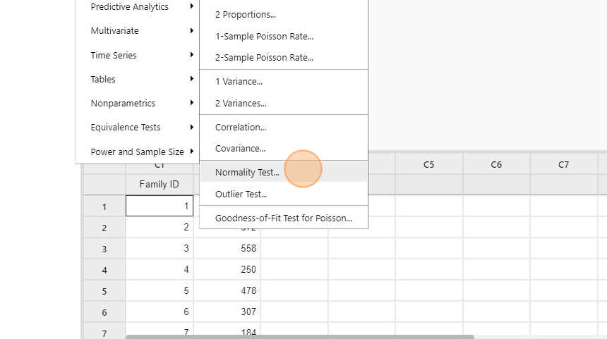
• A new window named “Normality Test” pops up.
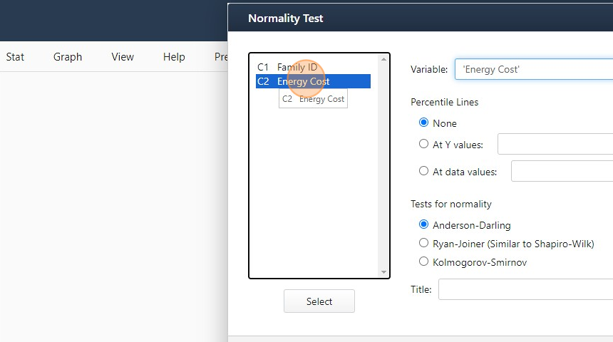
• Double Click “Energy Cost” to Select it as the “Variable”

  

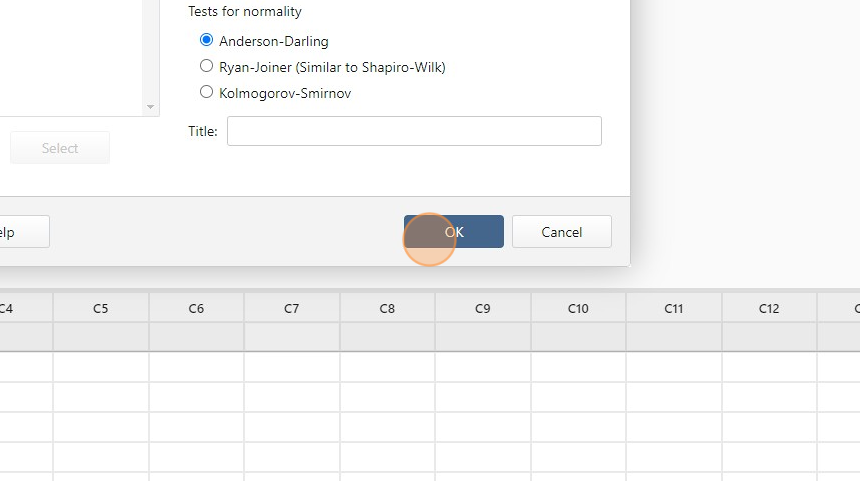
• Click “OK”

  

• The normality test results appear in the new window

  

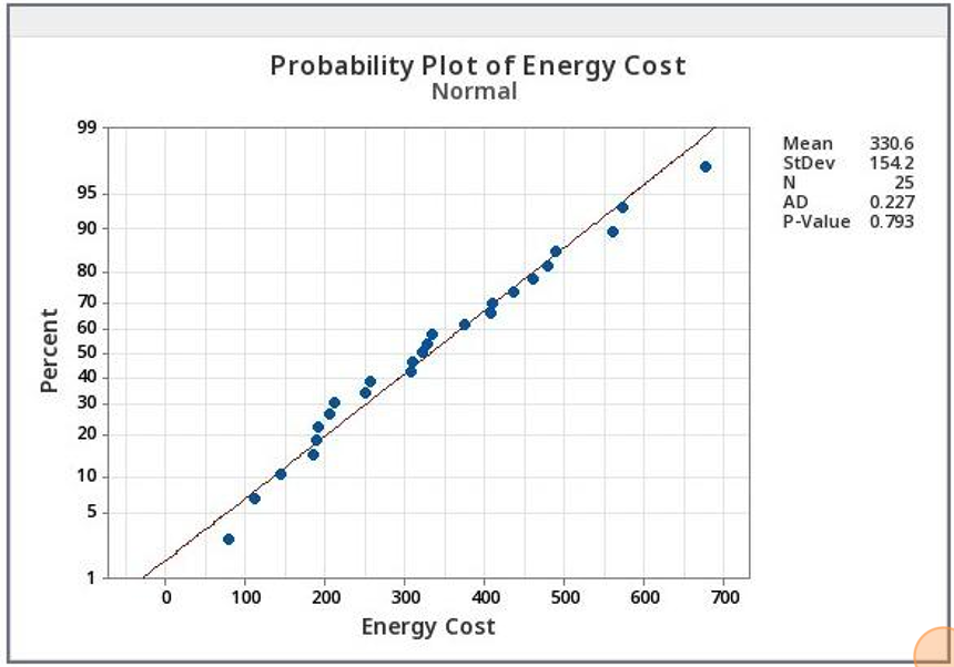
Conclusion: Check the p-value in the graph

Remember our assumptions?

• Null Hypothesis (H₀): The data are normally distributed.
• Alternative Hypothesis (H_a): The data are not normally distributed.
  • If the p-value is greater than the alpha level (0.05), we fail to reject the null hypothesis and claim that the data are normally distributed.
  • If the p-value is less than the alpha level (0.05), we reject the null hypothesis and claim that the data are not normally distributed.