One-Way ANOVA with JMP

What is One-Way ANOVA?

One-way ANOVA is a statistical method to compare the means of two or more populations.

• Null Hypothesis(H₀):): μ₁ = μ₂ ...= μ_k
• Alternative Hypothesis(H_a): At least one μ_i is different, where i is any value from 1 to k

It is a generalization of the two-sample t-test, since the two-sample t-test compares two population means, whereas the one-way ANOVA compares k population means (k ≥ 2).

Assumptions of One-Way ANOVA

• The sample data drawn from k populations are unbiased and representative
• The data of k populations are continuous
• The data of k populations are normally distributed
• The variances of k populations are equal

How ANOVA Works

ANOVA compares the means of different groups by analyzing the variances between and within groups. Let us say we are interested in comparing the means of three normally distributed populations. We randomly collected one sample for each population of our interest.

• Null Hypothesis(H₀): μ₁ = μ₂ = μ₃
• Alternative Hypothesis(H_a): One of the μ is different from the others

Based on the sample data, the means of the three populations might differ due to two sources of variation.

1. Variation between groups: non-random factors are leading to the variation.
2. Variation within groups results from random errors present within each group.

What we care about most is the variation between groups, since we are interested in whether the groups differ statistically. Variation between groups is the signal we want to detect, and variation within groups is the noise that corrupts the signal.

ANOVA is a modeling procedure, which means we use a model to predict results. To ensure the conclusions from ANOVA are reliable, we need to perform residual analysis.

Good residuals:

• Have a mean of zero
• Are normally distributed
• Are independent of each other
• Have equal variance

The difference between the actual and predicted result is called a residual or unexplained variation.

Use JMP to Run an ANOVA

Data File:  "OneWayANOVA.jmp"

• Null Hypothesis (H₀): μ₁ = μ₂ = μ₃ = μ₄ = μ₅
• Alternative Hypothesis (H_a): At least one of the five means is different from the others

Case study: We are interested in comparing average startup costs across five business types.

Step 1: Test whether the data for each level are normally distributed.

1. Click Analyze -> Distribution
2. Select “Cost” as “Y, Columns”
3. Select “Business” as “By”
   
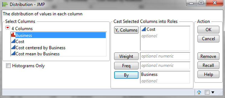
4. Click “OK”
5. Click on the red triangle button next to “Cost” in the Distribution page for “Business = X_i.”
6. Click Continuous Fit -> Normal
7. Click on the red triangle button next to “Fitted Normal.”
8. Select “Goodness of Fit”
   

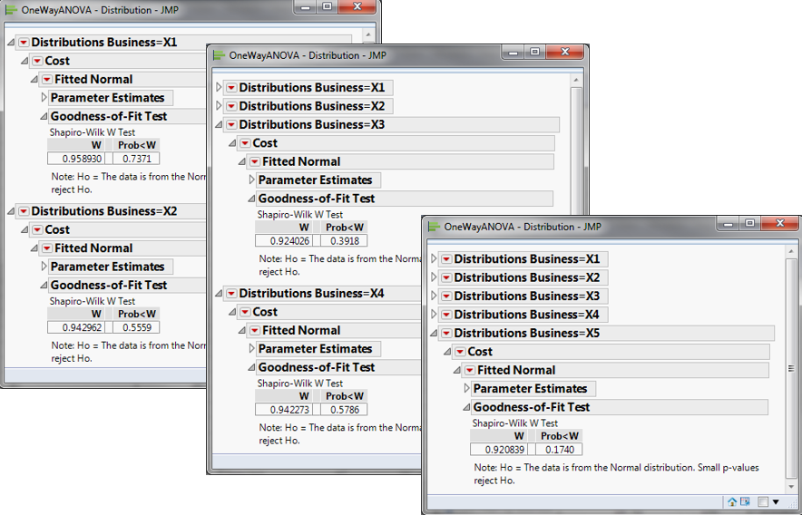
Notice that all p-values are greater than 0.05; therefore, we fail to reject the null hypothesis that the data are normally distributed.

• Null Hypothesis(H₀): The data are normally distributed
• Alternative Hypothesis(H_a): The data are not normally distributed

Since the p-values from the normality tests for the five data sets exceed the alpha level (0.05), we fail to reject the null hypothesis and conclude that the startup costs for any of the five businesses are normally distributed. If any of the five data sets are not normally distributed, we need to use alternative hypothesis-testing methods other than one-way ANOVA. In this example, all five data sets are normally distributed; however, if any were not, we would need to use another hypothesis test.

Step 2: Test whether the variance of the data for each level is equal to the variance of the other levels.

• Null Hypothesis(H₀):
• Alternative Hypothesis(H_a): at least one of the variances is different from the others

1. Click Analyze -> Fit Y by X
2. Select “Cost” as “Y, Response”
3. Select “Business” as “X, Factor”
   
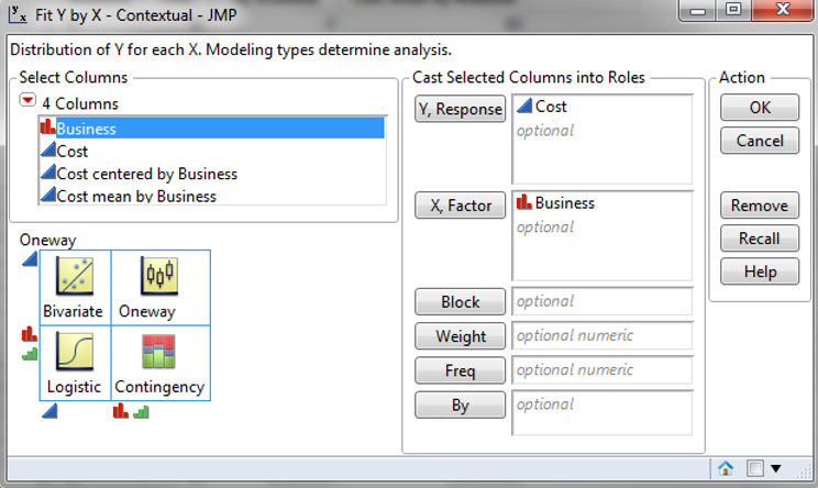
4. Click “OK”
5. Click on the red triangle button next to “One-Way Analysis of Cost by Business.”
6. Click “Unequal Variances”
   

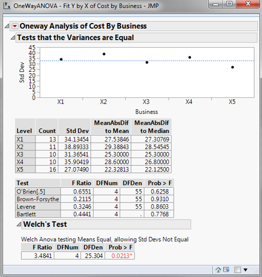
Use Bartlett’s test to test for equal variances across five levels, since there are more than two levels in the data and the data for each level are normally distributed. The p-value of Bartlett’s test is 0.777, greater than the alpha level (0.05), so we fail to reject the null hypothesis, and we claim that the variances of the five groups are equal. If the variances are not all equal, we need to use other hypothesis-testing methods than one-way ANOVA. If this test indicated that at least one variance differed, we would need to use a different hypothesis test to evaluate the group means.

Step 3: Test whether the mean of the data for each level is equal to the means of the other levels.

• Null Hypothesis(H₀): μ₁ = μ₂ = μ₃ = μ₄ = μ₅
• Alternative Hypothesis(H_a): at least one of the means is different from the others

1. Click on the red triangle button next to “One-Way Analysis of Cost by Business.”
2. Select “Mean/Anova”
   

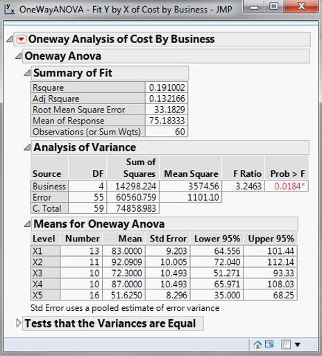
Since the p-value of the F test is 0.018, lower than the alpha level (0.05), the null hypothesis is rejected, and we conclude that at least one of the means of the five groups is different from the others.

Step 4: Save the residuals and predicted values after ANOVA. The predicted value for each level is the group mean.

1. Click on the red triangle button next to “One-way Analysis of Cost by Business.”
2. Select Save -> Save Residuals
3. Select Save -> Save Predicted
   

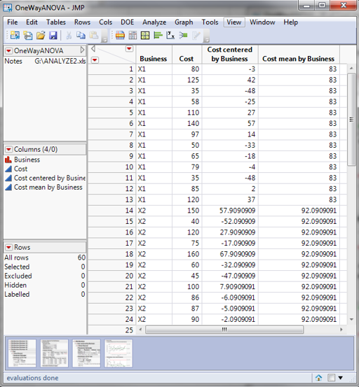
Step 5: Test whether the residuals are normally distributed with a mean of zero

1. Click Analyze -> Distribution
2. Select “Cost Centered by Business” as “Y, Columns”
   
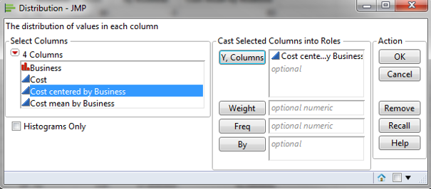
3. Click “OK”
4. Click on the red triangle button next to “Cost Centered by Business” in the Distribution page
5. Click Continuous Fit -> Normal
6. Click on the red triangle button next to “Fitted Normal.”
7. Select “Goodness of Fit”
   

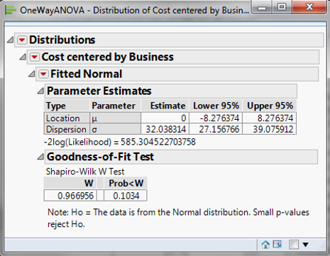
The p-value of the normality test is 0.1034, greater than the alpha level (0.05), and we conclude that the residuals are normally distributed. The mean of the residuals is 0.0000.

Step 6: Check whether the residuals are independent of each other.

• If the data are in time order, we can plot them in an IR chart to check for independence. When no data points on the IR chart fail any tests, the residuals are independent of each other.
• If the data are not in time order, the IR chart cannot provide a reliable conclusion about independence.

1. Click Analyze -> Quality & Process - > Control Chart -> IR
2. Select “Cost centered by Business” as “Process.”
   
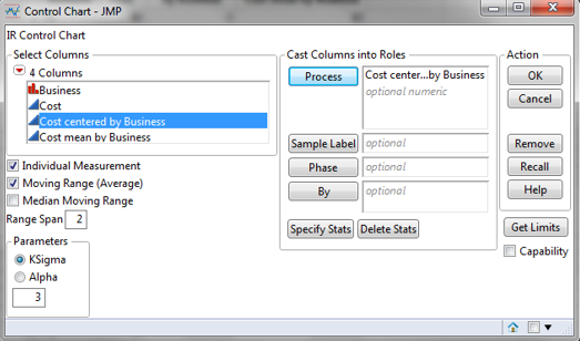
3. Click “OK”
4. Click on the red triangle button next to “Individual Measurements of Cost centered by Business.”
5. Select “Tests” -> “All Tests.”
   

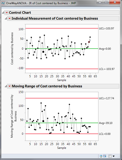
If the residuals are in time order, we can plot IR charts to check the independence. When no data points on the IR charts fail any tests, the residuals are independent of each other. If the residuals are not in time order, the IR charts cannot provide a reliable conclusion about independence.

Step 7: Plot residuals versus fitted values and check whether there is any systematic pattern.

1. Click Analyze-> Fit Y by X
2. Select “Cost centered by Business” as “Y, Columns.”
3. Select “Cost mean by Business” as “X”
   
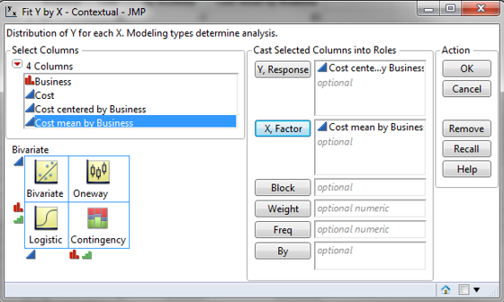
4. Click “OK”
   

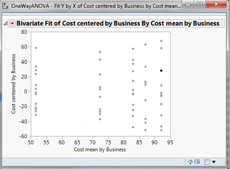
Model summary: The data points are evenly distributed across the five levels. Therefore, we can claim that the residuals have equal variances across all five levels.