Mann Whitney Testing with Minitab

What is the Mann Whitney Test?

The Mann Whitney test (also called Mann–Whitney U test or Wilcoxon rank-sum test) is a statistical hypothesis test to compare the medians of two populations that are not normally distributed. In a non-normal distribution, the median is the better representation of the center of the distribution.

• Null Hypothesis (H0): η₁ = η₂
• Alternative Hypothesis (Ha): η₁ ≠ η₂

Where:

•  η₁ is the median of one population
• η₂ is the median of the other population
• The null hypothesis is that the medians are equal, and the alternative is that they are not equal.

Mann Whitney Test Assumptions

• The sample data drawn from the populations of interest are unbiased and representative.
• The data of both populations are continuous or ordinal when the spacing between adjacent values is not constant. (Reminder: Ordinal data—A set of data is said to be ordinal if the values can be ranked or have a rating scale attached. You can count and order, but not measure, ordinal data.)
• The two populations are independent of each other.
• The Mann–Whitney test is robust for the non-normally distributed population.
• The Mann–Whitney test can be used when the shapes of the two populations’ distributions are different.

How Mann Whitney Test Works

Step 1:
Group the two samples from two populations (sample 1 is from population 1 and sample 2 is from population 2) into a single data set. Then, sort the data in ascending order from 1 to n, where n is the total number of observations.
Step 2:
Add up the ranks for all the observations from sample 1 and call it R1. Add up the ranks for all the observations from sample 2 and call it R2.
Step 3:
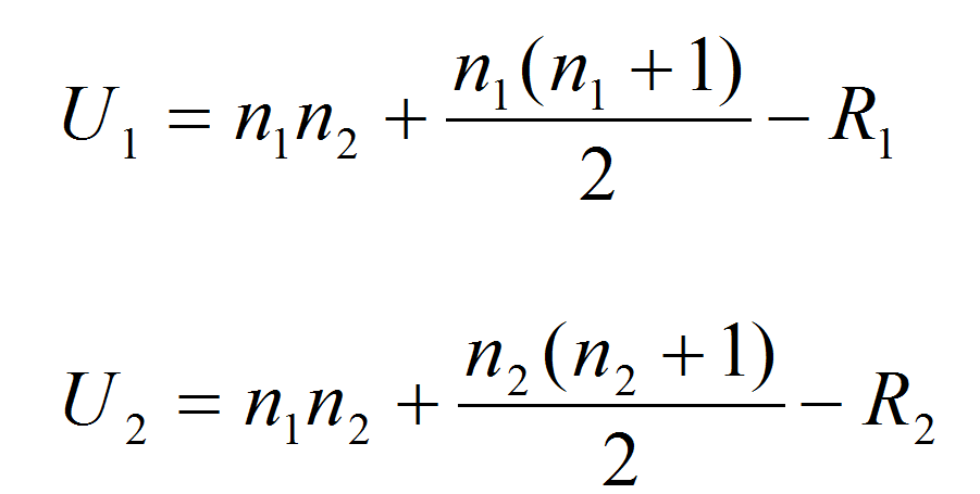
Calculate the test statistics

Where:

and where:

• η₁ and η₂ are the sample sizes
• R1 and R2 are the sum of ranks for observations from samples 1 and 2, respectively

Step 4:
Make a decision on whether to reject the null hypothesis.

• Null Hypothesis (H0): η₁ = η₂
• Alternative Hypothesis (Ha): η₁ ≠ η₂

If both of the sample sizes are smaller than 10, the distribution of U under the null hypothesis is tabulated.

• The test statistic is U, and by using the Mann–Whitney table, we would find the p-value.
• If the p-value is smaller than the alpha level (0.05), we reject the null hypothesis.
• If the p-value is greater than the alpha level (0.05), we fail to reject the null hypothesis.
• If both sample sizes are greater than 10, the distribution of U can be approximated by a normal distribution. In other words, (U-μ)/σ follows a standard normal distribution.

Z_calc=(U-μ)/σ

Where:

μ=(η₁ η₂)/2
σ=√(√(η₁ n_2 (η₁+η₂+1))/12)

If the sample sizes are greater than 10, then the distribution of U can be approximated by a normal distribution. The U value is then plugged into the formula here to calculate a Z statistic.
When |Zcalc| is greater than the Z value at α/2 level (e.g., when α = 5%, the z value we compare |Zcalc| to is 1.96), we reject the null hypothesis.

Use Minitab to Run a Mann–Whitney Test

Case study: We are interested in comparing customer satisfaction between two types of customers using a nonparametric (i.e., distribution-free) hypothesis test: Mann–Whitney test.
Data File: “Mann–Whitney” tab in “Sample Data.xlsx”

•  Null Hypothesis (H0): η₁ = η₂
• Alternative Hypothesis (Ha): η₁ ≠ η₂

Steps to run a Mann–Whitney Test in Minitab:

1. Un-stack the data into two separate columns:

• “Overall Satisfaction 1” for customer type = 1
• “Overall Satisfaction 2” for customer type = 2

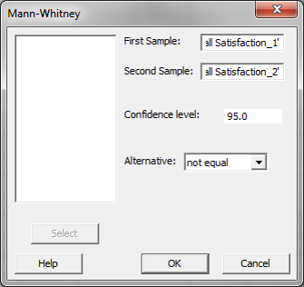
2. Click Stat → Nonparametrics → Mann–Whitney.
3. A new window named “Mann–Whitney” pops up.
4. Select “Overall Satisfaction 1” as the “First Sample.”
5. Select “Overall Satisfaction 2” as the “Second Sample.”
   
6. Click “OK.”
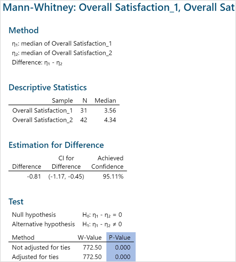
7. The Mann–Whitney test results appear in the session window.
   

Model summary: The p-value of the test is lower than the alpha level (0.05), so we reject the null hypothesis and conclude that there is a statistically significant difference between the overall satisfaction medians of the two customer types.