One Way ANOVA with SigmaXL

What is a One Way ANOVA with SigmaXL?

One way ANOVA with SigmaXL is a statistical method used to compare means of two or more populations. It is a generalized form of the two sample t-test since a two sample t-test compares two population means and one way ANOVA compares k population means where k ≥ 2.

• Null Hypothesis (H0): μ_1=μ_2=...=μ_k
• Alternative Hypothesis (Ha): At least one μi is different, where i is any value from 1 to k

Assumptions of One Way ANOVA

• The sample data drawn from k populations are unbiased and representative.
• The data of k populations are continuous.
• The data of k populations are normally distributed.
• The variances of k populations are equal.

How ANOVA Works

ANOVA compares the means of different groups by analyzing the variances between and within groups. Let us say we are interested in comparing the means of three normally distributed populations. We randomly collected one sample for each population of our interest.

• Null Hypothesis (H0): μ1 = μ2 = μ3
• Alternative Hypothesis (Ha): One of the μ is different from the others

Based on the sample data, the means of the three populations might look different because of two variation sources.

1. Variation between groups there are non-random factors leading to the variation between groups.
2. Variation within groups there are random errors resulting in the variation within each individual group.

What we care about the most is the variation between groups since we are interested in whether the groups are statistically different from each other. Variation between groups is the signal we want to detect and variation within groups is the noise which corrupts the signal.
ANOVA is a modeling procedure, which means we are using a model to try to predict results. To make sure the conclusions made in ANOVA are reliable, we need to perform residuals analysis.

• Good residuals:
• Have a mean of zero
• Are normally distributed
• Are independent of each other
• Have equal variance

The difference between the actual and predicted result is called a residual or unexplained variation.

Run an ANOVA with SigmaXL

Case study: We are interested in comparing the average startup costs of five kinds of business.

Data File: “One Way ANOVA” tab in “Sample Data.xlsx”

• Null Hypothesis (H0): μ1 = μ2 = μ3 = μ4 = μ5
• Alternative Hypothesis (Ha): At least one of the five means is different from others

Step 1: Test whether the data for each level are normally distributed.

1. Select the entire range of data (both “Business” and “Cost”)
2. Click SigmaXL -> Graphical Tools -> Histogram & Descriptive Statistics
3. A new window named “Histogram & Descriptive” pops up with the selected range pre-populated
   
4. Click “Next>>”
5. A new window named “Histogram & Descriptive” appears
6. Select “Cost” as “Numeric Data Variables (Y)” and “Business” as “Group Category (X1)”
   
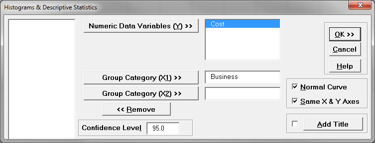
7. Click “OK>>”
8. The normality results appear in the new tab “Hist Descript (1)”
   

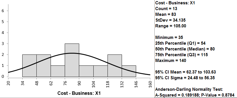
Shown above is one of the five outputs of the normality test. Upon review of all five tests, you’ll notice all of the p-values are greater than 0.05; therefore, we fail to reject the null hypothesis that the data are normally distributed.

Since the p-values of normality tests for the five data sets are higher than alpha level (0.05), we fail to reject the null hypothesis and claim that the startup costs for any of the five businesses are normally distributed. If any of the five data sets are not normally distributed, we need to use other hypothesis testing methods other than one-way ANOVA. In this example, all five data sets are normally distributed; however, if any of them were not normally distributed, we would need to use another hypothesis test.

Step 2: Test whether the variance of the data for each level is equal to the variance of other levels.

• Null Hypothesis(H₀):
• Alternative Hypothesis(H_a): at least one of the variances is different from others.

1. Select the entire range of data (both “Business” and “Cost”)
2. Click SigmaXL -> Statistical Tools -> Equal Variance Tests -> Bartlett’s Test (Since there are more than two levels in the data and the data of each level are normally distributed, we use Barlett’s test for testing the variances between the five levels.)
3. A new window named “Bartlett’s Test” pops up with the selected range pre-populated
   
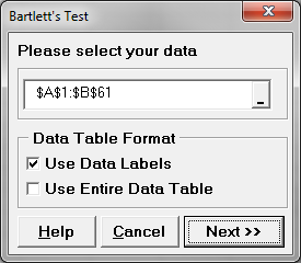
4. Click “Next>>”
5. A new window named “Bartlett’s Test” appears
6. Select “Cost” as the “Numeric Data Variable (Y)”
   Select “Business” as the “Group Category (X)”
   
7. Click “OK>>”
8. The results show up in the newly generated tab “Bartlett's Test (1)”
   

Use the Bartlett’s test for testing the equal variances between five levels in this case since there are more than two levels in the data and the data of each level are normally distributed. The p-value of Bartlett’s test is 0.776, greater than the alpha level (0.05), so we fail to reject the null hypothesis and we claim that the variances of five groups are equal. If the variances are not all equal, we need to use other hypothesis testing methods other than one-way ANOVA. If this test suggested that at least one variance was different, then we would need to use a different hypothesis test to evaluate the group means.

Step 3: Test whether the mean of the data for each level is equal to the means of other levels.

• Null Hypothesis(H₀): μ₁ = μ₂ = μ₃ = μ₄ = μ₅
• Alternative Hypothesis(H_a): at least one of the means is different from others

1. Select the entire range of the data (both “Business” and “Cost”)
2. Click SigmaXL -> Statistical Tools -> One-Way ANOVA & Means Matrix
3. A new window named “One-Way ANOVA” pops up with selected range pre-populated
   
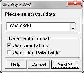
4. Click “Next>>”
5. A new window named “One-Way ANOVA & Means Matrix” appears
6. Select “Cost” as “Numeric Data Variable (Y)”
   Select “Business” as “Group Category (X)”
   Check the checkbox “Display ANOVA Table Details”
   
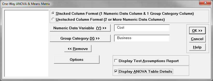
7. Click “OK>>”
8. The ANOVA results appear in the newly generated tab “One-Way ANOVA (1)”
   

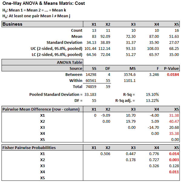
Model summary: Since the p-value of the F test is 0.018, lower than the alpha level (0.05), the null hypothesis is rejected and we conclude that the at least one of the means of the five groups is different from others.